Understanding Music Transformer

TLDR: This blog will discuss:
1 - Concepts discussed in the Music Transformer paper
2 - Background of Relative Attention, Relative Global Attention, Relative Local Attention
3 - Ideas in the paper to efficiently implement the above attention mechanisms
4 - Results on music generation

1 - Introduction

I personally suffer from a lot of pain points when I first try to understand the Music Transformer paper, especially the details in this paper about relative attention, local attention, and also the “skewing” procedure. To facilitate the understanding of Music Transformer, I decide to re-draw some of the diagrams, and explain each step in the model in a more detailed manner. I hope that this post could help more people understand this important work in music generation.

2 - Background of the Music Transformer

The Music Transformer paper, authored by Huang et al. from Google Magenta, proposed a state-of-the-art language-model based music generation architecture. It is one of the first works that introduce Transformers, which gained tremendous success in the NLP field, to the symbolic music generation domain.

The idea is as follows: by modelling each performance event as a token (as proposed in Oore et al.), we can treat each performance event like a word token in a sentence. Hence, we are able to learn the relationships between each performance event through self attention. If we train the model in an autoregressive manner, the model would also be able to learn to generate music , similar to training language models. From the demo samples provided by Magenta, it has been shown that Music Transformer is capable of generating minute-long piano music with promising quality, moreover exhibiting long-term structure.

Some related work of using Transformer architecture on generating music include MuseNet (from OpenAI), and also Pop Music Transformer. It is evident that the Transformer architecture would be the backbone of music generation models in future research.

For the basics of Transformers, we refer the readers who are interested to these links:

The Annotated Transformer from Harvard NLP;
Understanding and Applying Self-Attention for NLP Video;
Transformer Video by Hung-yi Lee, Mandarin version;
Transformers are Graph Neural Networks, a great blog post by Chaitanya Joshi.

3 - Transformer with Relative Attention

In my opinion, the Music Transformer paper is not only an application work, but its crux also includes optimization work on implementing Transformer with relative attention. We will delve into this part below.

The essence of Transformer is on self-attention: for an output sequence of the Transformer, the elements on each position is a result of “attending to” (weighted sum of, in math terms) the elements on each position in the input sequence. This is done by the following equation:
$$Attention(Q, K, V) = softmax(\frac{QK^T}{\sqrt{d}})V$$

where $Q, K, V$ represents the query, key and value tensors, each having tensor shape $(l, d)$, with $l$ and $d$ representing the sequence length and the number of dimensions used in the model respectively.

In Shaw et al., the concept of relative attention is proposed. The idea is to represent relative position representations more efficiently, to allow attention to be informed by how far two positions are apart in a sequence. This is an important factor in music as learning relative position representations help to capture structure information such as repeated motifs, call-and-response, and also scales and arpeggio patterns. Shaw et al. modified the attention equation as below:
$$Attention(Q, K, V) = softmax(\frac{QK^T + S^{rel}}{\sqrt{d}})V$$

The difference is to learn an additional tensor $S^{rel}$ of shape $(l, l)$. From the shape itself, we can see that the values $v_{ij}$ in $S^{rel}$ must be related to the relative distance of position $i$ and $j$ in length $l$.
In fact, we can also view a sequence as a fully connected graph of its elements, hence $S^{rel}$ can be seen as a tensor representing information about the edges in the graph.

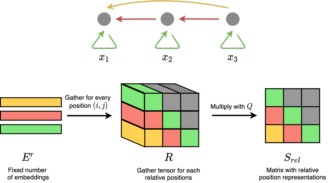
Figure 1: Relative attention in Shaw et al.. A sequence of 3 tokens is represented as a fully connected, backward directed graph, because commonly each node only attends the current steps and before.

How do we learn the values in $S^{rel}$? In Shaw et al., this is done by learning an extra weight tensor $R$ of shape $(l, l, d)$ – only 1 dimension extra as compared to $S^{rel}$. We can see it as having an embedding of dimension $d$, at each position in a distance matrix of shape $(l, l)$. The values $R_{i, j}$ means the embeddings which encode the relative position between position $i$ from query tensor, and position $j$ from key tensor. Here, we only discuss cases of masked self-attention without looking forward – only positions where $i \ge j$ is concerned because the model only attends to nodes that occur at the current time step or before.

After that, we reshape $Q$ into a $(l, 1, d)$ tensor, and multiply by $$S^{rel} = QR^T$$

However, this incurs a total space complexity of $O(L^2 D)$, restricting its application to long sequences. Especially in the context of music, minute-long segments can result in thousands of performance event tokens, due to the granularity of tokens used. Hence, Music Transformer proposes to “perform some algorithmic tricks” in order to obtain $S^{rel}$ in space complexity of $O(LD)$.

4 - Relative Global Attention

In Music Transformer, the number of unique embeddings in $E^r$ is assumed to be fixed. They used $l$ unique embeddings, ranging from the embedding for the furthest distance (which is $l - 1$, from first position to the $l^{th}$ position), to the embedding for the shortest distance (which is 0). Hence, the embedding for the “edge” between 1st and 3rd element, is the same as the embedding for the “edge” between 2nd and 4th element.

If we follow the assumptions made above, we can observe that the desired $S_{rel}$ can actually be calculated from multiplying $Q{E^{r}}^T$, only that further steps of processing are needed. From Figure 2 we can see that via some position rearrangement, we can get values of $S_{rel}$ from $Q{E^{r}}^T$.

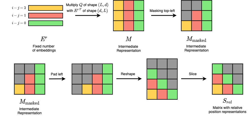
Figure 2: Relative attention procedure by Music Transformer.

The bottom row in Figure 2 is known as the “skewing” procedure for Music Transformer. Specifically, it involves reshaping a left-padded $M_\textrm{masked}$ and slice out the padded parts. The reshape function follows row-major ordering, which eventually rearranges each element to the right places which yields $S_{rel}$.

Hence, without using the gigantic $R$ tensor, and following the abovestated assumptions, a Transformer with relative attention only requires $O(LD)$ space complexity. Although both implementations result in $O(L^{2}D)$ in terms of time complexity, it is reported that Music Transformer implementation can run 6x faster.

4 - Relative Local Attention

Local attention, first coined in Luong et al and Image Transformer, means that instead of attending to every single token (which can be time costly and inefficient for extremely long sequences), the model only attends to tokens nearby at each time step. One way of implementation adopted in Image Transformer, which is also similar to the method discussed in Music Transformer, is the following: firstly, we divide the input sequence into several non-overlapping blocks. Then, each block can only attent to itself, and the block exactly before the current block (in Image Transformer, each block can attent to a memory block which includes the current block and a finite number of tokens before the block).

For simplicity, let’s start with an example of dividing the input sequence of 6 tokens into 2 blocks – Block 1 $[x_1, x_2, x_3]$, and Block 2 $[x_4, x_5, x_6]$. Hence, the attention components include: Block 1 $\leftrightarrow$ Block 1, Block 2 $\leftrightarrow$ Block 1, and Block 2 $\leftrightarrow$ Block 2, as shown in Figure 2.

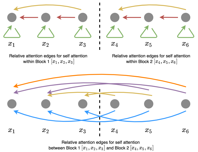
Figure 2: Relative local attention for a 6-token sequence, divided into 2 blocks .

The difference as compared to global attention can be observed when we have 3 blocks (and more). Then, if we set the local window to only include the current block and the previous block, then we no longer attent Block 3 $\leftrightarrow$ Block 1 as in global attention.

So, how can relative attention be introduced in local attention? Similarly, we want to include a matrix $S_{rel}$ which can capture relative position information, which similarly we can obtain the values from $Q{E^r}^T$ only with several different operations. To understand how should the operations be changed, we first see how does the desired $S_{rel}$ look like for 2 blocks:

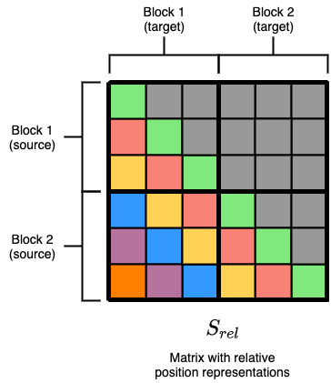
Figure 3: Desired relative position matrix .

From the above figure, we can analyze it according to 4 different factions of divided blocks. We can see that $S_{rel}$ output for Block 1 $\leftrightarrow$ Block 1, and Block 2 $\leftrightarrow$ Block 2 yields similar matrix as in relative global attention, hence the same reshaping and “skewing” procedure can be used. The only thing we need to change is the unmasked $S_{rel}$ output for Block 2 $\leftrightarrow$ Block 1, which will be the focus of discussion below.

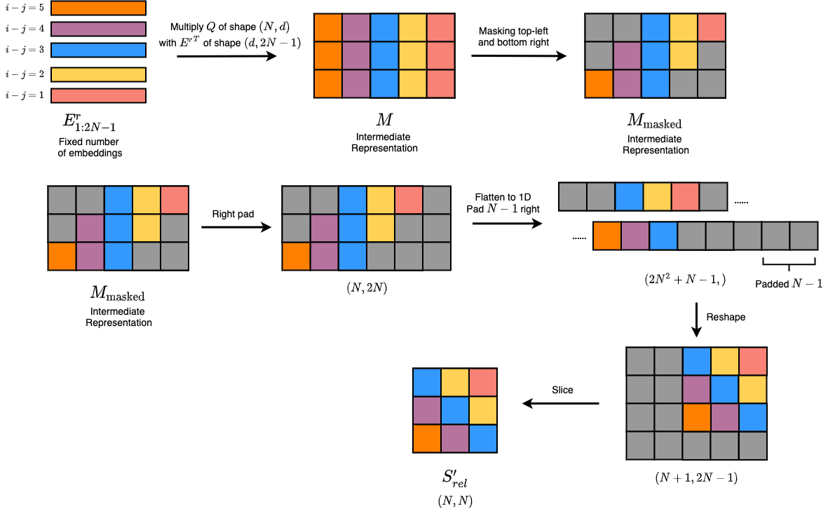
Figure 4: "Skewing" procedure for the unmasked part.

We denote $N$ to be the block length, hence in our simple example $N = 6 \div 2 = 3$. Following Figure 4, we can understand the changed procedure like this: first we gather the unique embeddings from $E^r$, only that this time we collect indices from $1$ to $2N-1$ (if we notice in the desired $S_{rel}$, these are the involved embeddings). This index range $[1:2N -1]$ is derived under the setting of attending only to the current and previous block. We similarly multiply $Q{E^r}^T_{1:2N-1}$, and this time we apply top-right and bottom left masks. Then, we pad one rightmost column, flatten to 1D, and reshape via row-major ordering. The desired position will be obtained after slicing.

One thing to note is that the discussion above omits the head indices – in actual implementation, one can choose to use the same $S_{rel}$ for each head, or learn separate $S_{rel}$ for different heads.

Note that this technique can be extended to larger numbers of divided blocks – generally, self-attending blocks can used the “skewing” procedure from relative global attention; non-self-attending blocks should use the latter unmasked “skewing” procedure. By this, we can succesfully compute $QK^T + S_{rel}$, with both shapes $(N, N)$, for each local attention procedure.

5 - Results

Finally, we take a quick glance on the results and comparisons made by the paper.

In general, relative attention achieves a better NLL loss as compared to vanilla Transformers and other architectures. Moreover, with more timing and relational information, it is evident that the results improved, and the authors also show that Music Transformer generates more coherent music with longer term of temporal structure. It seems like local attention does not really improve the results from global attention.

The main takeway from this work is clear: relative information does matter for music generation, and using relative attention provides more inductive bias for the model to learn these information, which corresponds to more evident musical structure and coherency. There are several attempts of using other Transformer variants (e.g. Transformer-XL in Pop Music Transformer), so we could probably foresee comparisons on different Transformer architectures for music generation in future.

6 - Code Implementation

The Tensorflow code of Music Transformer is open-sourced. Here, I link several portals that resembles with the important parts within the Music Transformer architecture:

The code is written using the Tensor2Tensor framework, so it might need some additional effort to set up the environment for execution. Ki-Chang Yang has implemented a very complete unofficial version in both Tensorflow and PyTorch, and I definitely recommend to check them out because it really helped me a lot on understanding the paper.