TLDR: This blog will discuss:
1 - Motivation of using semi-supervised learning in music modelling
2 - Two SSL frameworks based on latent generative models - Kingma et al and VaDE
3 - Applications of these frameworks on music-related tasks
1 - Introduction
In a previous post, we have discussed the usage of the popular VAE framework in symbolic music modelling tasks (surely, the framework can also be adapted to all kinds of music-related tasks). We have also seen that after training, the model jointly learns both inference and generation capabilities. Furthermore, by using extra techniques such as disentanglement, latent regularization, or using a more complex prior such as Gaussian mixture model, we observe how one or many meaningful, controllable latent space(s) could be learnt to support various downstream creative applications such as style transfer, morphing, analysis, etc.
In this post, we introduce the application of semi-supervised learning (SSL), which is very compatible with the VAE framework as we will see, to music modelling tasks. The (arguably) biggest pain-point in the music domain is that often times we do not have enough labelled data for all kinds of reasons – annotation difficulties, copyright issues, noise and high variance in annotations due to its subjective nature, etc. So, it will be good if the model can learn desirable properties with only limited amount of quality data.
2 - Why Semi-Supervised Learning?
The strengths and importance of SSL is especially evident in the music domain in my opinion. In particular, for abstract musical concepts which the labels definitely need human annotations (e.g. mood tags, arousal & valence, style, etc.), we can often observe two scenarios: (i) either the amount of labels is too little, which forbids the model to generalize well; or (ii) when the amount of labels start to scale, it becomes too noisy and deviated, due to the subjective nature of these annotations, which hinders the model from learning good representations.
Therefore, one of the solutions is to introduce SSL – we leverage the abundant amount of unlabelled data to learn common music representations, e.g. note, pitch, structure, etc., and we use only a very small set of quality labels (i.e. labels which are further filtered) to learn the desired abstract property. This further relates to the task of representation learning because we need to be able to learn reusable, high quality representations with only a small amount of labelled data in order achieve good results.
3 - Applying SSL to Deep Learning Models
SSL using Deep Generative Models
We start from one of the earliest papers that discuss SSL in deep learning models. In Kingma et al. the authors proposed a framework of using deep generative models for SSL, with graphical models as illustrated in Figure 1.
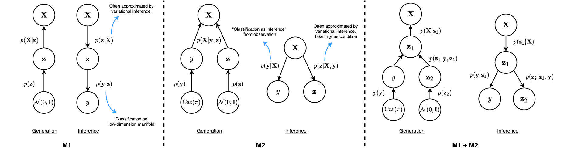
Figure 1: Graphical model of 3 formulations proposed in Kingma et al.
The generation components can be understood as how each model assumes each data point to be generated. \(\textrm{M1}\) resembles the idea of latent variable models, where a data point is generated from a latent prior, and further being projected to the observation space. \(\textrm{M2}\) is simply two strands of \(\textrm{M1}\) – one on the discrete class variable \(\textbf{y}\), and the other on the continuous latent \(\textbf{z}\). \(\textrm{M2}\) can also be viewed as a disentanglement model, if we understand it as learning separate spaces for labels in \(\textbf{y}\), and residual information in \(\textbf{z}\) (e.g. writing styles in MNIST). \(\textrm{M1} + \textrm{M2}\) is generally a hierachical combination of both.
On the other hand, all exact posterior \(p(\textbf{z} | \textbf{X})\) are approximated using variational inference by introducing a new distribution \(q_{\phi}(\textbf{z} | \textbf{X})\). The posterior can also be called the inference component, as we are inferring the latent distributions from the observations.
The posterior for \(\textrm{M1}\) is evident to be \(q_{\phi}(\textbf{z} | \textbf{X})\), and the model employs a separate classifier (e.g. an SVM) to predict \(\textbf{y}\) from the low-dimension manifold \(\textbf{z}\), which could be encoded with more meaningful representations and yields better classification accuracy. For \(\textrm{M2}\), the authors parameterized the posterior to be \(q_{\phi}(\textbf{z} | \textbf{X}, \textbf{y}) = q_{\phi}(\textbf{z} | \textbf{X}) \cdot q_{\phi}(\textbf{y} | \textbf{X})\), which the class labels are inferred directly from \(\textbf{X}\) using a separate Gaussian inference network.
So, how does the objective function look like if we want to train the model in a semi-supervised manner?
For \(\textrm{M1}\), we are basically training a VAE, so the objective function is:
$$E_{\textbf{z}\sim q_{\phi} (\textbf{z}|\textbf{X})}[\log p_\theta(\textbf{X}|\textbf{z})] - \mathcal{D}_{KL}(q_\phi(\textbf{z}|\textbf{X}) || p(\textbf{z}))$$ Additionally, the label classifier is trained separated on only labelled data. Hence, the posterior learnt will serve as a feature extractor used to train the label classifier.
For \(\textrm{M2}\), we need to consider two cases: if label is present (supervised), then the objective function is very similar to the VAE objective function, other than an additional given \(\textbf{y}\):
$$\mathcal{L(\textbf{X}, y)} = E_{\textbf{z}\sim q_\phi(\textbf{z}|\textbf{X}, y)} [ \log p_\theta(\textbf{X}|\textbf{z}, y) + \log p_\theta(y) + \log p(\textbf{z}) - \log q_\phi(\textbf{z}|\textbf{X}, y)] \\ = E_{\textbf{z}\sim q_\phi(\textbf{z}|\textbf{X}, y)}[\log p_\theta(\textbf{X}|\textbf{z}, y)] - \mathcal{D}_{KL}(q_\phi(\textbf{z}|\textbf{X}, y) || p(\textbf{z}))$$ If label is not present (unsupervised), then we marginalize over all possibilities of class labels as below:
$$\mathcal{U(\textbf{X})} = \displaystyle\sum_{y} q_\phi(y | \textbf{X}) \cdot [ \mathcal{L(\textbf{X}, y)} - \mathcal{D}_{KL}(q_\phi(y|\textbf{X}) || p(y)) ] \\ = \displaystyle \sum_y q_\phi(y | \textbf{X}) \cdot \mathcal{L(\textbf{X}, y)} + \mathcal{H}(q_\phi(y|\textbf{X}))$$
where the additional entropy term \(\mathcal{H}(q_\phi(y|\textbf{X}))\) pushes the distribution to conform to a multinomial prior distribution. Additionally, to improve the classification capability of \(q_\phi(y|\textbf{X})\), a classification loss (e.g. cross-entropy loss) can be added during the supervised scenario. The extension to \(\textrm{M1} + \textrm{M2}\) is then straigtforward by combining the loss terms of both models. All inference and generation parameters, \(\phi\) and \(\theta\), are parameterized using neural networks, with some popular choices in the music domain like 1D or 2D CNNs, RNNs, attention networks etc.
Variational Deep Embedding (VaDE)
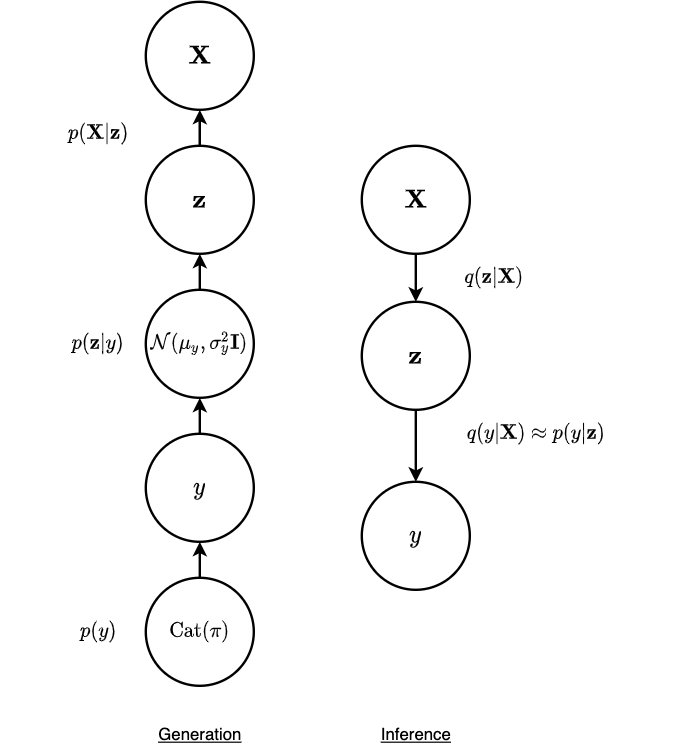
Figure 2: Graphical model of VaDE.
VaDE employs the idea of unsupervised and generative approach on clustering. Hence as shown in Figure 2, the graphical model is a hierachical structure from \(\textbf{X} \rightarrow \textbf{z} \rightarrow y\) for the inference component. One can relate this to discrete representation learning using VAE with a Gaussian mixture prior – after inferring the latent variable \(\textbf{z}\), the variable is assigned to a particular cluster with index \(y\). Hence, it is straightforward that the objective function is the ELBO extended to a mixture-of-Gaussian scenario:
$$E_{\textbf{z}\sim q_{\phi} (\textbf{z}, y|\textbf{X})}[\log p_\theta(\textbf{X}|\textbf{z})] - \mathcal{D}_{KL}(q_\phi(\textbf{z}, y| \textbf{X}) || p(\textbf{z}, y))$$ The second KL term regularizes the latent embedding \(z\) to lie on the mixture-of-Gaussians manifold. Similarly, we can introduce both supervised and unsupervised scenario in this case: when labels are present (supervised), the KL term is written as:
$$ - \mathcal{D}_{KL}(q_\phi(\textbf{z}|\textbf{X}, y) || p(\textbf{z}|y))$$
and when labels are not present (unsupervised), we similarly marginalize over all possibilities of class labels, as we have done for the \(\textrm{M2}\) model before:
$$ - \displaystyle \sum_y q_\phi(y|\textbf{X}) \cdot \mathcal{D}_{KL}(q_\phi(\textbf{z}|\textbf{X}) || p(\textbf{z}|y)) + \mathcal{H}(q_\phi(y|\textbf{X}))$$
Comparison
Here, we can see that both frameworks by Kingma et al. and VaDE share a lot of similarities. Firstly, both frameworks are latent variable models, and make use of the generative approach. To achieve semi-supervised capabilities, both frameworks adopt the strategy to marginalize over all classes. In fact, if we look close at the inference component in \(\textrm{M1} + \textrm{M2}\), the left strand actually resembles the inference graphical model of VaDE. The main difference in both frameworks lie in the prior distribution. Kingma et al. model 2 separate distributions, which is a multinomial distribution for \(y\) and a standard Gaussian for \(\textbf{z}\), whereas VaDE integrates both into a single mixture-of-Gaussians.
4 - Applications
The SSL frameworks above are suitable to be applied in music domain for two reasons: firstly, by training the model we can get both discriminative capability for analysis / feature extraction, and generation capability for all kinds of creative synthesis. Secondly, we can rely on the generation component to learn meaningful musical representations from unlabelled data. Through training the model to generate outputs that are similar to the data distribution, we want the model to learn useful, reusable musical features which can be easily regularized or separated by leveraging only a small amount of labels.
An example discussed for music generation is by Ferreira et al on generating music with sentiment. Obviously, the amount of unlabelled music is massive, and sentiment-labelled data is extremely scarce. The authors adopted the model from Radford et al on generating reviews with sentiment. The model used is an \(\textrm{mLSTM}\) which takes in the previous tokens as input, and is trained to predict the next token in an autoregressive manner. The intermediate representation from \(\textrm{mLSTM}\) are used for sentiment classification. Thi model can actually be interpreted as a variant of \(\textrm{M1}\), with the intermediate representation from \(\textrm{mLSTM}\) as \(\textbf{z}\), and a separate logistic regressor is used to predict \(y\) from \(\textbf{z}\).
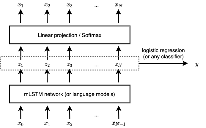
Figure 3: Sentiment fine-tuning on mLSTM by Ferreira et al.
Another example is by Luo et al on disentangling pitch and timbre for audio recordings on playing single notes. The model proposed basically resembles with VaDE, with an additional disentanglement added to learn separate spaces for pitch and timbre. The authors studied the results of pitch and timbre classification by using increasing amount of labelled data. An additional advantage demonstrated is that we can learnt both discrete and continuous representations for both pitch and timbre – discrete representations are intuitive for analysis, as pitch and timbre are normally in discrete terms; however, the continuous representations are useful for applications such as gradual timbre morphing. The representations between two instruments could serve as a blend of both which could help discover new types of instrument timbre styles.
Another two strong examples demonstrating the strength of SSL-VAE frameworks (which also helped me understand a lot on SSL-VAE applications), though not in the music domain, is by the Tacotron team. Two of their papers explore similar ideas to VaDE and Kingma et al to involve hierarchical modelling and semi-supervised learning for realistic text-to-speech generation. One of the examples is demonstrated on affect conditioning, which is again often a scarely-labelled scenario, yet the authors are able to achieve outstanding results on speech synthesis.
Conclusion
With the rise in popularity of using latent variable models for music modelling, it is intuitive that by incorporating the frameworks mentioned above, these models can be extended easily to support SSL capabilities. Perhaps some interesting questions to ask are: what is the lower-bound of the amount of data we need to achieve good results with SSL-VAE architectures? How much could we further improve on the generation component to “self-supervisedly” learn good representations, and reduce the necessity of using more labels? Can the training go even further to purely unsupervised scenarios? These are indeed exciting research problems waiting to be solved.
For the fundamental framework papers, please refer to the list below:
- Semi-supervised Learning with Deep Generative Models
- Variational Deep Embedding: An Unsupervised and Generative Approach to Clustering
- Learning Disentangled Representations with Semi-Supervised Deep Generative Models