
TLDR: This blog will discuss:
1 - A very brief introduction on short-time Fourier transform
2 - How spectrogram conversion can be implemented using CNNs (based on nnAudio)
1 - Introduction
Recently, I have wanted to understand more about the audio domain in music signal processing. The obvious start will be to understand from time-frequency representations first, namely spectrograms. My wonderful colleague Raven Cheuk had released a GPU audio processing named nnAudio last year, which implements fast spectrogram conversions on GPU with 1D convolution nets, and I decided to further understand this connection between STFT and 1D CNNs.
2 - Short Time Fourier Transform (STFT)
First, we discuss the case for discrete Fourier transform (DFT), which converts a given audio signal of length \(L\) into a vector \(X_{DFT}\) of size \(N\), where \(N\) is the number of frequency bins (commonly, we set \(L = N\) for convenience in calculations). DFT basically tells the frequency distribution of the audio signal across multiple frequency bins. The equation can be written as:
$$X_{DFT}[n] = \displaystyle\sum_{l=1}^{L} x[l] \cdot e^{-i \cdot 2 \pi \cdot n \cdot \frac{l}{N}}$$
However, the output DFT does not contain any time-related information. Hence, the solution is to chop the audio signal into multiple windows, apply DFT on each of them, and concatenate the vector outputs along the time axis. This results in the discrete short-time Fourier transform (STFT), which converts a given audio signal of length \(L\) into a time-frequency representation of shape \((N, T)\). \(N\) is the number of frequency bins, and \(T\) is the number of time steps, whereby for each time step a DFT operation is performed within a window of length \(L_{\textrm{w}}\) (similarly, \(L_{\textrm{w}} = N\) for convenience in calculations), and the number of steps is determined by how much the window is slided (hop length, \(H\)) to finish “sweeping” the audio signal.
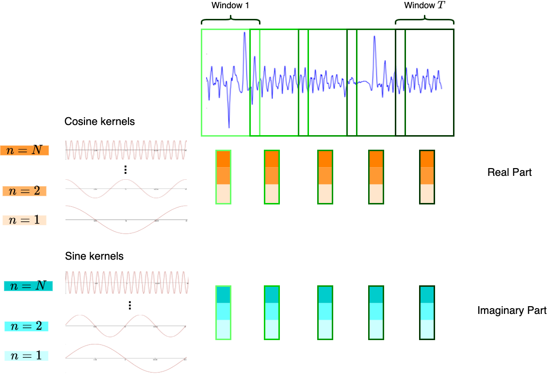
Figure 1: Discrete Short-Time Fourier Transform.
Given an audio signal \(x\), a complex-form spectrogram \(X\) which is the output of STFT is expressed by:
$$X[n, t] = \displaystyle\sum_{l=1}^{L_w} x[t \cdot H + l] \cdot w[l] \cdot e^{-i \cdot 2 \pi \cdot \frac{n}{N} \cdot l}$$
We can further use Euler’s formula to expand \(e^{-i \cdot 2 \pi \cdot \frac{n}{N} \cdot l}\) into \(\cos(2 \pi \cdot \frac{n}{N} \cdot l) - i\sin(2 \pi \cdot \frac{n}{N} \cdot l)\). The term \(w[l]\) is an additional window function which helps to distribute spectral leakage according to the needs of the application.
From Figure 1, we can already see the resemblance between 1D CNNs and STFT conversions. Understanding from the perspective of convolution networks, we can interpret Figure 1 as having \(N\) cosine and sine “filters” respectively, and perform 1D convolution on the audio signal, whereby the stride is exactly of the hop length \(H\).
3 - Inverse STFT
Can inverse STFT be implemented in terms of CNNs as well? In fact, this torch-stft library implemented inverse STFT using 1D transposed convolutional nets. However, here I would like to portray an implementation using 2D convolution nets instead.
If we put together the equations of discrete DFT and inverse DFT (with window function) as below:
$$X_{DFT}[n] = \displaystyle\sum_{l=1}^{L} x[l] \cdot w[l] \cdot e^{-i \cdot 2 \pi \cdot n \cdot \frac{l}{N}} \\ x[l] = \frac{1}{N \cdot w[l]} \displaystyle\sum_{n=1}^{N} X_{DFT}[n] \cdot e^{i \cdot 2 \pi \cdot n \cdot \frac{l}{N}}$$
we can observe that both equations appear to be very related, and the terms are seemingly interchangeable. This also means that if we implement STFT using 1D convolutions, we can perform inverse STFT using the same cosine and sine “filters”, as the Euler term stays the same.
As \(X_{DFT}\) is in complex form, we can observe that the multiplication with the Euler term results in:
$$(X_{real} + i X_{imag})(\cos \phi + i \sin \phi) \\ = (X_{real}\cos \phi - X_{imag}\sin \phi) + i(X_{real}\sin \phi + X_{imag}\cos \phi)$$ and as the input signal \(x\) is a real-value signal, we should observe that the values lie within the real part of the output, and \(X_{real}\sin \phi + X_{imag}\cos \phi = 0\).
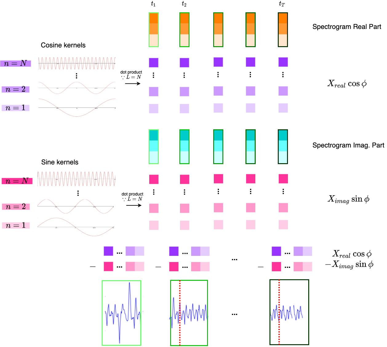
Figure 2: Inverse Short-Time Fourier Transform with the same convolution filters.
Since STFT is just a temporal version of DFT, we can perform inverse DFT using the above-stated method on each time step. Figure 2 illustrates the above-stated method using the same convolution filters. The only difference is that, since now the input is a 2D spectrogram, we have to perform 2D convolution. Hence, we can interpret the operation as performing 2D convolution using the cosine / sine filters of shape \((N, 1)\) on the spectrogram with shape \((N, T)\) with stride \((1, 1)\).
The final output will be the segments of the original audio, with overlapped redundant parts due to the windows overlapping each other during STFT (see the parts to the left of the red dashed line in Figure 2). We can easily observe that other than the first segment, all segments have a starting overlapped segment of length \(L_w - H\), hence by removing these starting overlapped segments and concatenating all segments together we can reconstruct the original audio signal.
4 - Code Implementation
The above-stated methods are implemented in nnAudio using PyTorch, I provide the portals as follows: